Big O Notation: Understanding Algorithm Complexity
Data Structures and Algorithms: Part 1
Writing software involves more than finding a solution that produces the correct result. We also need to consider how efficiently that solution performs, particularly as the amount of data it processes increases.
An algorithm that works perfectly with ten records might become inefficient when processing ten thousand or even a million records. Understanding how an algorithm's performance changes as its input grows is an important part of building scalable software.
This is where Big O notation becomes useful.
Big O provides a mathematical way to describe how an algorithm's resource requirements grow relative to its input size. It helps developers reason about performance, compare different approaches to solving the same problem, and identify potential bottlenecks before they become problems.
In this article, we'll explore what Big O notation means, examine common complexity classes, and use practical C# examples to understand how to analyse algorithm efficiency.
1. What is Big O notation?
Big O notation describes the asymptotic upper bound of a function that represents an algorithm's resource requirements as its input size increases.
In simpler terms, it helps us understand how an algorithm behaves when the amount of data it processes becomes larger.
Consider two approaches to finding a particular value in a collection:
- The first approach examines every element until it finds the target.
- The second approach uses a more efficient searching strategy that repeatedly eliminates half of the remaining elements.
Both approaches might produce the correct answer, but their performance characteristics are different, particularly when dealing with large collections.
Big O allows us to express and compare these differences mathematically.
Understanding input size (n)
In algorithm analysis, we commonly use the variable n to represent the size of an algorithm's input.
For example:
- An array containing 10 elements has an input size of n = 10.
- An array containing 1,000 elements has an input size of n = 1,000.
- An array containing 1 million elements has an input size of n = 1,000,000.
The value of n allows us to reason about how an algorithm's resource requirements change as its input grows.
Input size does not always represent the number of elements in an array. Depending on the problem, it could represent the number of characters in a string, the number of nodes in a graph, or the number of records being processed.
For problems involving multiple inputs, we might use different variables, such as n and m, to represent their respective sizes.
What does asymptotic growth mean?
Asymptotic analysis focuses on how an algorithm behaves as its input size becomes very large.
Rather than measuring the exact execution time in milliseconds, we examine the rate at which its resource requirements grow.
For example, consider two algorithms:
- Algorithm A performs approximately n operations.
- Algorithm B performs approximately n² operations.
When n is small, the difference might be insignificant. As n increases, however, the number of operations required by Algorithm B grows much faster.
Big O allows us to focus on these growth patterns without getting distracted by constant factors and implementation-specific details.
It is worth noting that Big O technically describes an upper bound, not exclusively worst-case performance. In everyday software engineering discussions, it is frequently used to describe worst-case complexity, but the distinction matters when analysing algorithms precisely.
2. Understanding common Big O complexity classes
There are several complexity classes that developers frequently encounter when analysing algorithms. Let's explore them individually, starting with constant time.
O(1): Constant time
An algorithm has constant time complexity when its number of operations does not grow with the size of its input.
Consider accessing an element in an array using its index:
int[] numbers = { 10, 20, 30, 40, 50 };

int result = numbers[2];
Regardless of whether the array contains five elements or five million elements, accessing an element using its index takes a constant amount of time.
The operation does not need to examine the elements before the requested index.
Therefore, the time complexity is:
O(1): Constant time
Constant time does not necessarily mean that an operation takes only one machine instruction. It means that its operation count does not grow with the input size.
Other examples include assigning a value to a variable and accessing an element in a hash table under normal lookup assumptions.
O(log n): Logarithmic time
An algorithm has logarithmic time complexity when its resource requirements grow logarithmically as the input size increases.
A common example is binary search.
Binary search works by repeatedly dividing a sorted collection into two halves until the target value is found or there are no remaining elements to examine.
Consider searching for the number 42 in a sorted collection containing 16 elements. Rather than examining every element, binary search compares the target with the middle element and eliminates half of the remaining collection with each comparison.
The search space develops approximately as follows:
| Step | Remaining elements |
|---|---|
| Initial collection | 16 |
| First comparison | 8 |
| Second comparison | 4 |
| Third comparison | 2 |
| Fourth comparison | 1 |
Instead of examining all 16 elements, the algorithm needs at most approximately four divisions to narrow the search down to one element.
Here is a C# implementation:
public static int BinarySearch(
    int[] numbers,
    int target)
{
    int left = 0;
    int right = numbers.Length - 1;

    while (left <= right)
    {
        int middle = left + (right - left) / 2;

        if (numbers[middle] == target)
            return middle;

        if (numbers[middle] < target)
            left = middle + 1;
        else
            right = middle - 1;
    }

    return -1;
}
Each iteration eliminates approximately half of the remaining search space. This gives binary search a worst-case time complexity of:
O(log n): Logarithmic time
An important requirement is that the collection must be sorted before binary search can be applied. Sorting an unsorted collection also has a cost that needs to be considered.
O(n): Linear time
An algorithm has linear time complexity when the number of operations grows proportionally to the size of its input.
Consider a method that searches through an array to find a particular value:
public static int LinearSearch(
    int[] numbers,
    int target)
{
    for (int i = 0; i < numbers.Length; i++)
    {
        if (numbers[i] == target)
            return i;
    }

    return -1;
}
In the worst case, the algorithm must examine every element before determining whether the target exists.
For an array containing:
- 10 elements, it might examine 10 elements.
- 100 elements, it might examine 100 elements.
- 1,000 elements, it might examine 1,000 elements.
The number of operations grows proportionally with the input size.
Therefore, its worst-case time complexity is:
O(n): Linear time
Linear complexity is not necessarily inefficient. Sometimes, examining every element is unavoidable, depending on the problem being solved.
O(n log n): Linearithmic time
Linearithmic time complexity combines linear and logarithmic growth.
A common example is Merge Sort, which uses a divide-and-conquer approach to sort a collection.
The algorithm works in three main stages:
- Divide the collection into smaller sections.
- Continue dividing until each section contains a single element.
- Merge the sections back together in sorted order.
The collection is divided approximately log₂(n) times. At each level, merging requires work proportional to n.
This results in a time complexity of:
O(n log n): Linearithmic time
The following is a simplified C# implementation using an auxiliary array:
public static void MergeSort(int[] numbers)
{
    int[] buffer = new int[numbers.Length];

    Sort(numbers, buffer, 0, numbers.Length - 1);
}

private static void Sort(
    int[] numbers,
    int[] buffer,
    int left,
    int right)
{
    if (left >= right)
        return;

    int middle = left + (right - left) / 2;

    Sort(numbers, buffer, left, middle);
    Sort(numbers, buffer, middle + 1, right);

    Merge(numbers, buffer, left, middle, right);
}

private static void Merge(
    int[] numbers,
    int[] buffer,
    int left,
    int middle,
    int right)
{
    int i = left;
    int j = middle + 1;
    int k = left;

    while (i <= middle && j <= right)
    {
        if (numbers[i] <= numbers[j])
            buffer[k++] = numbers[i++];
        else
            buffer[k++] = numbers[j++];
    }

    while (i <= middle)
        buffer[k++] = numbers[i++];

    while (j <= right)
        buffer[k++] = numbers[j++];

    for (int index = left; index <= right; index++)
        numbers[index] = buffer[index];
}
Merge Sort has O(n log n) time complexity in its best, average, and worst cases. This implementation also requires O(n) auxiliary space for the buffer.
We'll explore sorting algorithms, including Merge Sort, in greater detail in a dedicated article later in this series.
O(n²): Quadratic time
An algorithm has quadratic time complexity when the number of operations grows proportionally to the square of its input size.
A common example is a nested loop where both loops iterate over the same collection.
Consider:
public static void PrintPairs(int[] numbers)
{
    for (int i = 0; i < numbers.Length; i++)
    {
        for (int j = 0; j < numbers.Length; j++)
        {
            Console.WriteLine(
                $"{numbers[i]}, {numbers[j]}");
        }
    }
}
For every element in the collection, the inner loop iterates through the entire collection.
If the collection contains:
- 10 elements, the method performs 100 iterations.
- 100 elements, the method performs 10,000 iterations.
- 1,000 elements, the method performs 1,000,000 iterations.
The total number of iterations is n multiplied by n.
Therefore, the time complexity is:
O(n²): Quadratic time
Quadratic algorithms can become expensive as input sizes increase. However, nested loops do not automatically mean O(n²). The complexity depends on how many times each loop executes and how those iterations relate to the input size.
O(2ⁿ): Exponential time
An algorithm has exponential time complexity when its operation count grows exponentially with the input size.
A classic example is a recursive solution that calculates Fibonacci numbers without storing previously calculated results.
public static int Fibonacci(int n)
{
    if (n <= 1)
        return n;

    return Fibonacci(n - 1)
         + Fibonacci(n - 2);
}
Each call can generate two additional recursive calls, resulting in a growing tree of calculations. Many of the same Fibonacci values are calculated repeatedly.
The recurrence relation for this implementation is:
T(n) = T(n - 1) + T(n - 2) + O(1)
Its tighter asymptotic time complexity is Θ(φⁿ), where φ (phi) is the golden ratio, approximately 1.618. O(2ⁿ) is a valid but less precise upper-bound description.
There is another problem with this implementation: integer overflow.
In C#, the int type has a maximum value of 2,147,483,647. Fibonacci(46) still fits within this limit, but Fibonacci(47) does not. In the default unchecked arithmetic context, the result overflows rather than producing the correct Fibonacci number.
The implementation, therefore, has both a performance limitation and a numerical limitation. Even before integer overflow becomes relevant, repeated calculations make this approach increasingly expensive.
Techniques such as memoisation and dynamic programming can significantly improve its performance by avoiding repeated calculations. We'll explore these techniques in a future article.
3. Comparing common complexity classes
Now that we've explored the different complexity classes, let's compare how they behave as input sizes increase.
The following graph plots their growth functions for input sizes ranging from 1 to 50.
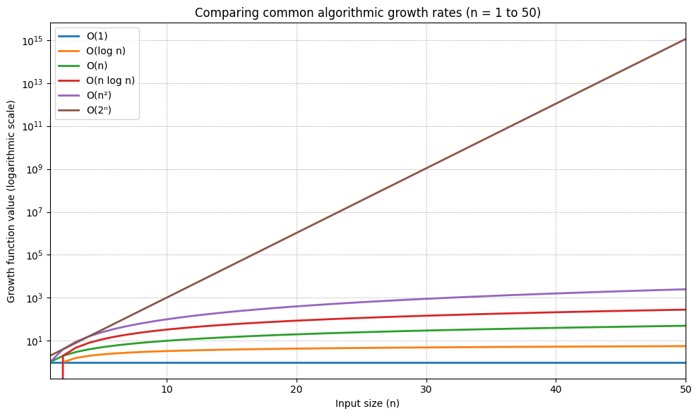
The vertical axis uses a logarithmic scale because exponential growth would otherwise dominate the graph and make the slower-growing functions difficult to distinguish.
The graph illustrates an important principle: algorithms with lower asymptotic growth rates generally scale better as their input sizes increase.
| Complexity | Name | General behaviour |
|---|---|---|
| O(1) | Constant | Does not grow with input size |
| O(log n) | Logarithmic | Grows slowly |
| O(n) | Linear | Grows proportionally |
| O(n log n) | Linearithmic | Faster growth than linear |
| O(n²) | Quadratic | Grows rapidly |
| O(2ⁿ) | Exponential | Grows extremely rapidly |
However, Big O alone does not tell us which implementation will execute faster for every possible input size. Constant factors, memory allocation, hardware and implementation details can also influence actual performance.
For example, an algorithm with O(n) complexity might be faster than an O(log n) algorithm for a particular small input because the latter has a higher fixed overhead.
Big O is most useful for understanding scalability, not predicting exact execution times.
4. How to analyse Big O complexity
Understanding the different complexity classes is useful, but being able to identify them in code is even more important.
There are several practical principles that help when analysing algorithms.
Rule 1: Ignore constant factors
Consider the following method:
public static void PrintNumbers(int[] numbers)
{
    for (int i = 0; i < numbers.Length; i++)
    {
        Console.WriteLine(numbers[i]);
        Console.WriteLine(numbers[i]);
    }
}
The loop executes two operations per element, but its growth is still proportional to n.
Its complexity is:
O(2n) = O(n)
Big O focuses on how performance grows as input size increases, rather than the exact number of operations performed.
Rule 2: Ignore lower-order terms
Consider an algorithm that performs n² operations followed by n additional operations.
Its complexity can be represented as:
O(n² + n)
As n becomes larger, the quadratic term dominates the linear term. We therefore simplify the expression to:
O(n²)
This makes it easier to compare algorithms based on their dominant growth rates.
Rule 3: Sequential operations are added
Consider two loops that execute one after the other:
public static void ProcessNumbers(int[] numbers)
{
    for (int i = 0; i < numbers.Length; i++)
    {
        Console.WriteLine(numbers[i]);
    }

    for (int i = 0; i < numbers.Length; i++)
    {
        Console.WriteLine(numbers[i]);
    }
}
Each loop has O(n) complexity.
The combined complexity is:
O(n) + O(n) = O(2n) = O(n)
Rule 4: Nested loops are multiplied
Consider the following example involving users and permissions:
public static void ProcessUsers(
    User[] users,
    Permission[] permissions)
{
    foreach (var user in users)
    {
        foreach (var permission in permissions)
        {
            Console.WriteLine(
                $"{user.Name}: {permission.Name}");
        }
    }
}
The outer loop iterates over n users, while the inner loop iterates over m permissions for every user.
The total number of iterations is:
O(n × m)
This is an important distinction. It is only O(n²) if both collections grow proportionally with the same input size.
Nested loops can also produce other complexity classes. For example:
public static void ProcessNumbers(int n)
{
    for (int i = 0; i < n; i++)
    {
        for (int j = 1; j < n; j *= 2)
        {
            Console.WriteLine($"{i}, {j}");
        }
    }
}
The outer loop executes n times. The inner loop doubles j on each iteration, giving it O(log n) complexity.
The combined complexity is:
O(n × log n)
The key is to examine how each loop progresses, rather than simply counting the number of nested loops.
Rule 5: Repeatedly reducing the input often produces logarithmic complexity
Consider the following loop:
public static void ReduceInput(int n)
{
    while (n > 1)
    {
        n /= 2;
    }
}
Every iteration reduces the input size by half.
The number of iterations required to reach one is proportional to log₂(n).
Therefore, the time complexity is:
O(log n)
5. Time complexity vs. space complexity
So far, we've primarily focused on how the number of operations grows as input size increases.
However, performance is not only about execution time. We also need to consider memory consumption.
Time complexity describes how the number of operations performed by an algorithm grows relative to its input size.
Space complexity describes how the memory requirements of an algorithm grow relative to its input size.
When analysing space complexity, it is useful to distinguish between total space and auxiliary space.
- Total space complexity considers the overall memory requirements, including the input and additional memory.
- Auxiliary space complexity focuses specifically on the additional memory an algorithm uses while executing, excluding its input.
Auxiliary space is particularly useful when comparing implementations because it shows how much extra memory an algorithm requires.
Consider the following method:
public static int SumNumbers(int[] numbers)
{
    int total = 0;

    foreach (int number in numbers)
    {
        total += number;
    }

    return total;
}
The method visits every element in the array exactly once.
Its time complexity is O(n).
However, it only uses a fixed amount of additional memory for the total and number variables.
Its auxiliary space complexity is O(1).
Now consider another implementation:
public static int[] DoubleNumbers(int[] numbers)
{
    int[] result = new int[numbers.Length];

    for (int i = 0; i < numbers.Length; i++)
    {
        result[i] = numbers[i] * 2;
    }

    return result;
}
This method also visits every element once, giving it O(n) time complexity.
However, it creates a new array containing n elements.
Its auxiliary space complexity is O(n).
This distinction matters because an algorithm can be efficient in terms of execution time but require a significant amount of additional memory.
6. Understanding best-case, average-case and worst-case complexity
Another important aspect of algorithm analysis is understanding that an algorithm can behave differently depending on the input it receives.
Let's return to our linear search implementation.
Suppose we are searching for a value in an array containing 1,000 elements.
There are three possible scenarios.
Best case
The target is the first element in the array. The algorithm finds it immediately.
Time complexity: O(1).
Average case
The target is somewhere in the middle of the array, or the algorithm needs to examine a substantial portion of the collection. Assuming the target is equally likely to appear at any position, the expected number of comparisons is approximately n/2.
Time complexity: O(n).
Worst case
The target is the final element, or it does not exist in the array. The algorithm must examine every element.
Time complexity: O(n).
These scenarios help us understand how an algorithm behaves under different conditions.
In practice, developers frequently focus on worst-case complexity because it provides an upper-bound perspective on how much work an algorithm might require.
However, average-case analysis is also valuable when the expected distribution of inputs is understood.
One technical distinction worth remembering: best-case, average-case, and worst-case describe the scenarios being analysed. Big O describes an asymptotic upper bound on the resulting function. They are related concepts, but they are not interchangeable.
7. Applying Big O in real software development
Big O is not just an academic concept or something developers need to memorise for coding interviews. It has practical applications when designing and maintaining software.
Consider a helpdesk application that needs to retrieve a support ticket using its identifier.
One approach might be to iterate through a collection of tickets until the matching identifier is found.
public static SupportTicket? FindTicket(
    List<SupportTicket> tickets,
    int ticketId)
{
    foreach (var ticket in tickets)
    {
        if (ticket.Id == ticketId)
            return ticket;
    }

    return null;
}
This approach has O(n) worst-case lookup complexity because it might need to examine every ticket.
Alternatively, we could use a dictionary that maps ticket identifiers to ticket objects.
Dictionary<int, SupportTicket> tickets = new();

tickets.Add(101, new SupportTicket());
tickets.Add(102, new SupportTicket());

if (tickets.TryGetValue(102, out var ticket))
{
    Console.WriteLine("Ticket found");
}
Under normal hash table assumptions, dictionary lookups have O(1) average time complexity.
The .NET documentation describes Dictionary<TKey, TValue> retrieval as close to O(1), with performance depending partly on the quality of the hashing algorithm.
This illustrates an important engineering decision: choosing an appropriate data structure can significantly influence application performance.
However, that does not mean a dictionary is always the right choice. We also need to consider memory consumption, ordering requirements, insertion costs and the operations our application performs most frequently.
The objective is not simply to choose the data structure with the lowest Big O complexity. It is to choose one that best satisfies the requirements of the problem.
8. Common misconceptions about Big O
Before concluding, there are a few misconceptions worth addressing.
- Big O measures execution time in seconds. It describes how resource requirements grow with input size, not actual execution time.
- O(1) always means faster than O(n). Constant factors and implementation overhead can make an O(n) algorithm faster for particular input sizes.
- Every nested loop has O(n²) complexity. The complexity depends on the number of iterations and how the loops relate to the input size.
- Big O always means worst-case complexity. Big O describes an asymptotic upper bound. It can be used to analyse different cases.
- An algorithm with better Big O is always the better choice. Memory consumption, input sizes, implementation complexity and practical performance also matter.
9. Key takeaways
Big O notation is one of the fundamental tools developers use to reason about algorithm efficiency.
The most important concepts to take away from this article are:
- Big O describes the asymptotic growth of an algorithm's resource requirements as its input size increases.
- The variable n commonly represents the size of an algorithm's input.
- O(1), O(log n) and O(n) describe constant, logarithmic and linear growth respectively.
- O(n log n), O(n²) and O(2ⁿ) describe progressively faster growth rates.
- Time complexity and space complexity measure different resource requirements.
- Best-case, average-case and worst-case analysis help us understand an algorithm under different input conditions.
- Choosing appropriate data structures and algorithms can significantly influence application performance.
Most importantly, Big O encourages developers to think beyond whether their code produces the correct result. It encourages us to consider how well our solutions perform as the problems they solve become larger.
10. Test your understanding
Try answering these questions before moving on.
- What is the time complexity of accessing an element in an array using its index?
- Why does binary search have logarithmic time complexity?
- What is the time complexity of two sequential loops, each iterating over the same array?
- What is the difference between time complexity and space complexity?
- Why is O(n²) generally less scalable than O(n)?
- Can an O(1) algorithm execute more slowly than an O(n) algorithm for a particular input size?
- What is the difference between worst-case analysis and Big O notation?
- What is the time complexity of nested loops where the outer loop executes n times and the inner loop executes log n times?
Practical exercise
Write three C# methods:
- A method that finds the largest number in an integer array.
- A method that checks whether an array contains duplicate values using nested loops.
- A method that checks whether an array contains duplicate values using a
HashSet<int>.
For each method:
- Explain how it works.
- Analyse its time complexity.
- Analyse its auxiliary space complexity.
- Compare the two approaches to finding duplicates.
The goal is not simply to identify the correct complexity class. It is to develop the habit of examining code and reasoning about the resources it requires.
This article is part of a Data Structures and Algorithms series exploring the fundamental concepts, techniques, and problem-solving approaches used in software development.
Comments
Join the discussionNo comments yet. Be the first to comment.